Group sizes, durations and aggreation
The analysis of real-world face-to-face data is often based on the analysis of networks in terms of disconnected groups — the group sizes, their lifetimes and the contact durations distributions. Furthermore, an aggregated static network is often used to analyze the social structure. In the following we show how to compute and analyze these observables easily.
Base analysis function
To do a complete measurement of the group size histograms,
the group life time distributions, the contact and
inter-contact distributions, and the aggregated weighted
network use tacoma.api.measure_group_sizes_and_durations()
result = tc.measure_group_sizes_and_durations(temporal_network)
The returned object is an instance of _tacoma.group_sizes_and_durations.
Group sizes
We define the group size distribution \(N_g(t)\) describing the number of groups of size \(g\) at time \(t\). Note that the group size distribution is restricted by
The time-dependent group size distribution is saved in two ways.
For edge_lists
For each edge list, a size
histogram as a dictionary of (int, int)-pairs is saved in the
attribute result.size_histograms. The key is the group size
\(g\) and the value is number of its occurences.
For edge_changes
A single group size histogram is computed for the initial edge list.
Then, for each edge changing event,
a dictionary is saved in result.size_histogram_differences, where
keys are the group size \(g\) and the corresponding value is
the change of occurences in comparison to the network’s previous state.
Note
Since evaluating the size histograms might be heavy on memory, you can omit the detailed computation using
result = tc.measure_group_sizes_and_durations(
                    temporal_network,
                    ignore_size_histogram=True
                    )
Averaged size distribution
The average group size distribution
is saved in result.aggregated_size_histogram, a list of floats
where the g-th entry contains the average number of groups of size
g. Note that this implies that the 0-th entry is always equal to 0.
You can easily get a numpy.ndarray of group sizes g and corresponding
average number of groups of this size N_g using the function
tacoma.tools.group_size_histogram().
g, N_g = tc.group_size_histogram(result)
Note that this function returns values for non-zero occurences only.
If you are just interested in the mean group size, use
tacoma.tools.mean_group_size()
mean_g = tc.mean_group_size(result)
Number of groups
At all times, the number of seperated components (groups) is given by
and thus the mean number of components over time is
It can be computed with tacoma.tools.mean_number_of_groups().
mean_c = tc.mean_number_of_groups(result)
Coordination number
The coordination number \(n\) of a single node is defined as the group size this node is part of, as was first done in a study by Zhao, Stehlé, Bianconi, and Barrat. The probability distribution of the coordination number is given by the group size distribution \(N_g\) as
It can also be interpreted as the probability of a single node to be in a group of size \(n\).
The mean coordination number \(\left\langle n \right\rangle\) can be computed as
mean_n = tc.mean_coordination_number(result)
Analysis
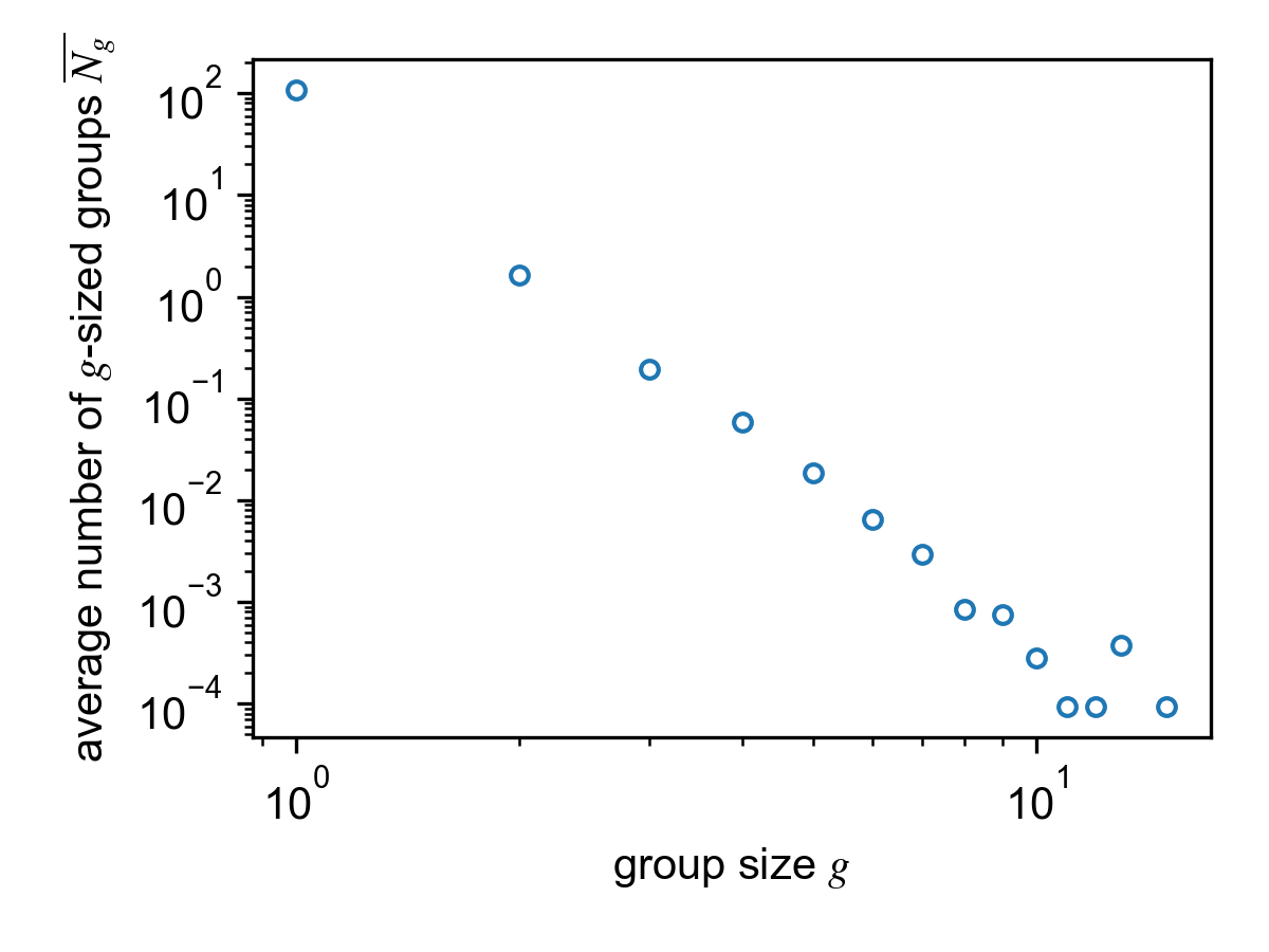
Plot a distribution of group sizes as
from tacoma.analysis import plot_group_size_histogram
import matplotlib.pyplot as pl

ht09 = tc.load_sociopatterns_hypertext_2009()
result = tc.measure_group_sizes_and_durations(ht09)

fig, ax = pl.subplots(1,1)
plot_group_size_histogram(result, ax)
pl.show()

Average group size histogram for the SocioPatterns Hypertext 09 dataset.
Durations
Group durations
A group is initiated as soon as an event leads to a change in members. The duration of this group is defined as the time it takes until the next event at which the constituents of the group changes.
All durations of groups of size \(g\) are saved in
result.group_durations[g] (hence, result.group_durations[0]
is always empty).
Groups which were active at \(t_0\) are not considered in the measurement since we do not know when they were initiated, so including them in the analysis would skew the distribution. Likewise, groups which are still active at \(t_\mathrm{max}\) are omitted for the same reason.
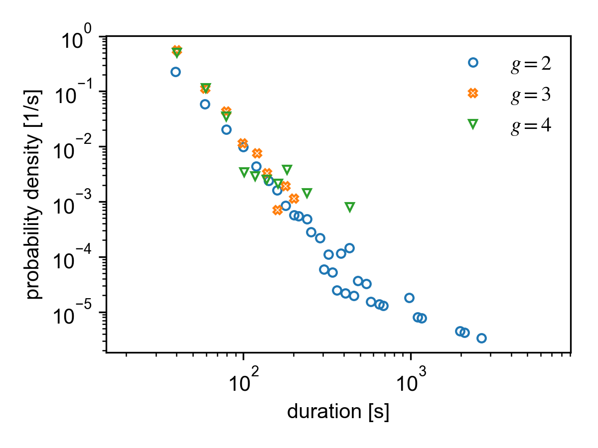
The durations can be analyzed using tacoma.analysis.plot_group_durations().
from tacoma.analysis import plot_group_durations
import matplotlib.pyplot as pl

ht09 = tc.load_sociopatterns_hypertext_2009()
result = tc.measure_group_sizes_and_durations(ht09)

fig, ax = pl.subplots(1, 1)
plot_group_durations(result, ax, max_group=4, time_unit='s')

pl.show()

Duration distribution of different group sizes for the SocioPatterns Hypertext 09 dataset.
(Inter-) Contact durations
The durations of all contacts is saved in result.contact_durations.
However, contacts which were active at \(t_0\) are omitted since
we do not know when they started, so including them in the analysis would
skew the distribution. Likewise, contacts which are still active at
\(t_\mathrm{max}\) are omitted for the same reason.
The inter-contact duration of a node is defined as the time a node spends
alone (i.e. in a group of size \(g=1\)). Hence, all inter-contact
durations are saved in result.group_durations[1].
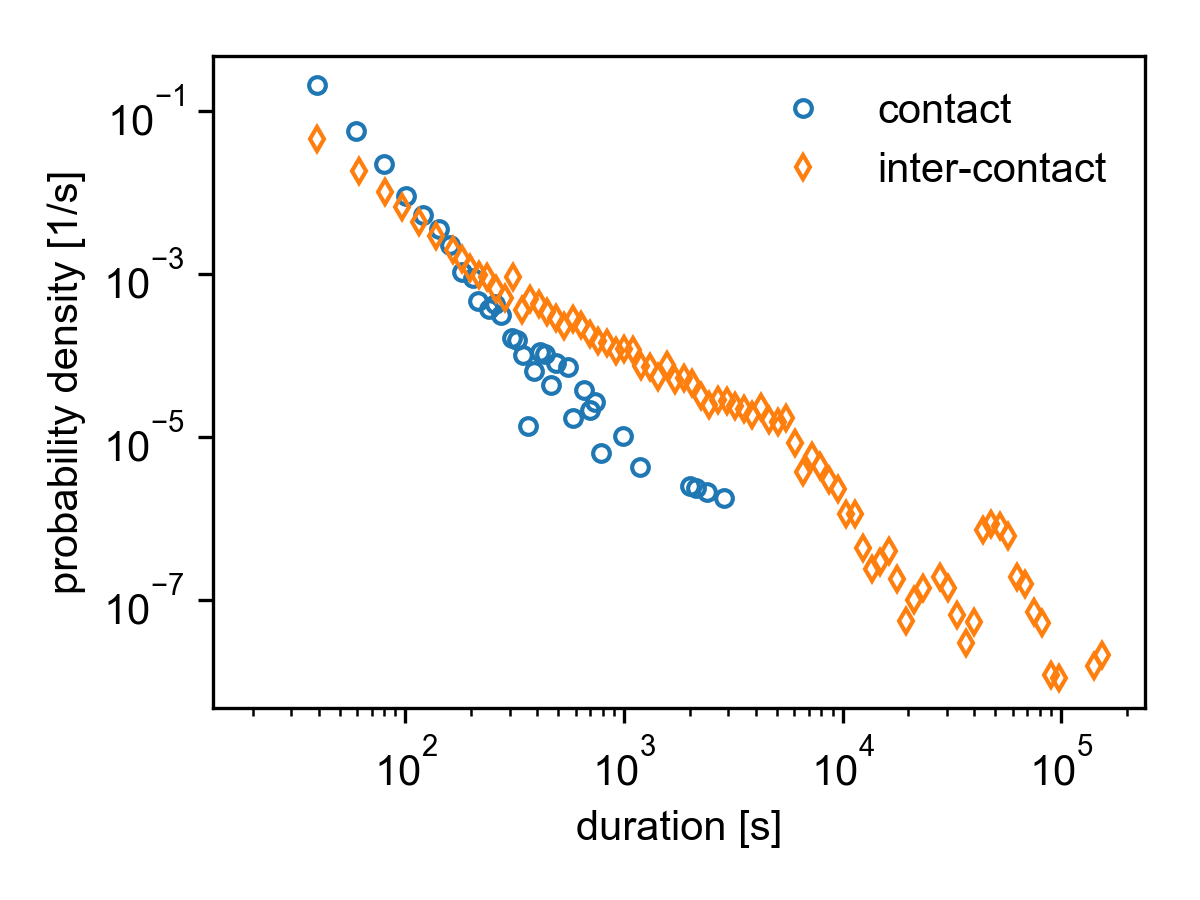
The contact and inter-contact durations can be analyzed using
tacoma.analysis.plot_group_durations().
from tacoma.analysis import plot_contact_durations
import matplotlib.pyplot as pl

ht09 = tc.load_sociopatterns_hypertext_2009()
result = tc.measure_group_sizes_and_durations(ht09)

fig, ax = pl.subplots(1, 1, figsize=(4,3))
plot_contact_durations(result, ax, time_unit='s')
pl.show()

Contact and inter-contact distributions for the SocioPatterns Hypertext 09 dataset.
Aggregated network
The aggregated network
is given as a dictionary in result.aggregated_network. Each key
is a pair of ints, representing the edge \((i, j)\), the
corresponding value is \(W_{ij}\).
If you just want the aggregated network without the other results,
use tacoma.api.aggregated_network().