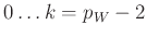
... notwendig.¹

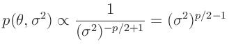
Zu den notwendigen Voraussetzungen für ein lineares Modell gibt es unterschiedliche Auffassungen:
Martin (2012) Seite 145: Insbesondere ist die Annahme nicht notwendig, dass die Fehler der Messwerte normalverteilt sind.
James (2006) Seite 186: Es werden keine Annahmen über die Verteilung der Daten $\bm{y}$ gemacht.
Nollau (1975) setzt schon bei der Herleitung des linearen Modells für die $\epsilon_i$ unabhängige normalverteilte Zufallsgrößen voraus.

.
.
.
.
.
.
.
.
.
.
.
.
.
.
.
.
.
.
.
.
.
.
.
.
.
.
.
.
.
.

... Erwartungswert²

Im Unterschied zu Martin (2012)(Seite 145), Fahrmeir (2009)(Seite 62) und Nollau (1975)(Seite 134) verwendet James (2006) in diesem Zusammenhang im Kapitel 8.4 (Seite 183ff) anstelle von $\bm{\mathrm{E}}[y_i]$ den Ausdruck $\bm{\mathrm{E}}[y_i,\bm{\theta}]$.

.
.
.
.
.
.
.
.
.
.
.
.
.
.
.
.
.
.
.
.
.
.
.
.
.
.
.
.
.
.

... Konstante³

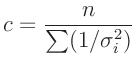
Bevington (2003) wählt im Kapitel 11 für die Gewichte (Gleichung (11.2) Seite 194, Gleichung (11.32) Seite 203 sowie auf Seite 215) den Ausdruck:

$$p_i = \frac{1/\sigma_i^2}{(1/n)\sum(1/\sigma_i^2)} = \frac{n}{\sum(1/\sigma_i^2)}\; \frac{1}{\sigma_i^2}$$

Daraus folgt für die Konstante c:

$$c = \frac{n}{\sum(1/\sigma_i^2)}$$

Dies entspricht einer Normalisierung der Gewichtsfaktoren auf deren Mittelwert.

.
.
.
.
.
.
.
.
.
.
.
.
.
.
.
.
.
.
.
.
.
.
.
.
.
.
.
.
.
.

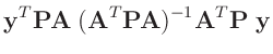
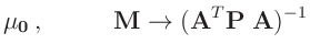
... damit:⁴

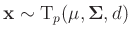
Nach Fahrmeir (2009)( Seite 463 ) gilt für die Linearkombination eines Zufallsvektors $\bm{X}$ mit einer geeignet dimensionierten Matrix $\bm{A}$ und einem geeignet dimensionierten Vektor $\bm{b}$:

$$\bm{\mathrm{E}}[\bm{A}\bm{X} +\bm{b}] = \bm{A}\,\bm{\mathrm{E}}[\bm{X}] +\bm{b}$$

$$\bm{\mathrm{Cov}}[\bm{A}\bm{X} +\bm{b}] = \bm{A}\,\bm{\mathrm{Cov}}[\bm{X}]\,\bm{A}^T$$

Damit ergibt sich mit $\bm{\Sigma}=\bm{\mathrm{Cov}}[\bm{y}]$ :

$$\bm{\mathrm{Cov}}[\widehat{\bm{\theta}}] = \bm{\mathrm{Cov}}[(\bm{A}^T\bm{P}\bm{A})^{-1}\,\bm{A}^T\bm{P}\,\bm{y}]$$

$$= (\bm{A}^T\bm{P}\;\bm{A})^{-1}\bm{A}^T\bm{P}\, \bm{\Sigma}\, \left((\bm{A}^T\bm{P}\;\bm{A})^{-1}\bm{A}^T\bm{P}\right)^T$$

Mit $\bm{\Sigma}=\widehat{\sigma^2}\,\bm{P}^{-1}$ folgt daraus:

$$\bm{\mathrm{Cov}}[\widehat{\bm{\theta}}] = \widehat{\sigma^2}\,(\bm{A}^T\bm{P}\;\bm{A})^{-1}(\bm{A}^T\bm{P}\bm{A})(\bm{A}^T\bm{P}\;\bm{A})^{-1}$$

$$= \widehat{\sigma^2}\,(\bm{A}^T\bm{P}\;\bm{A})^{-1}$$

da die Matrizen $\bm{P}$ und $\bm{A}^T\bm{P}\;\bm{A}$ symmetrisch sind.

.
.
.
.
.
.
.
.
.
.
.
.
.
.
.
.
.
.
.
.
.
.
.
.
.
.
.
.
.
.

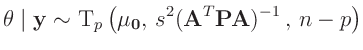
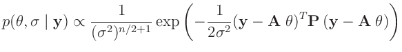
... Maximum-Likelihood-Schätzung⁵

Die Maximum-Likelihood-Schätzung

$$\widehat{\sigma^2}=\frac{1}{n}\,\widehat{\bm{\epsilon}}^T\bm{P}\widehat{\bm{\epsilon}}$$

ist nicht erwartungstreu. Im allgemeinen wird sie deswegen durch die Restringierte Maximum-Likelihood-Schätzung

$$\widehat{\sigma^2}=\frac{1}{n-p}\,\widehat{\bm{\epsilon}}^T\bm{P}\widehat{\bm{\epsilon}}$$

ersetzt. (Fahrmeir (2009) Seite 94, Wakefield (2013) Seite 44 ff.)

.
.
.
.
.
.
.
.
.
.
.
.
.
.
.
.
.
.
.
.
.
.
.
.
.
.
.
.
.
.

... Signifikanzniveau⁶

Im Praktikum wird meist mit $(1 \sigma)$-Fehlerintervallen gearbeitet. Das zugehörige Signifikanzniveau ist $68.2689\%$, woraus $\alpha = 31.7311\%$ folgt.

.
.
.
.
.
.
.
.
.
.
.
.
.
.
.
.
.
.
.
.
.
.
.
.
.
.
.
.
.
.

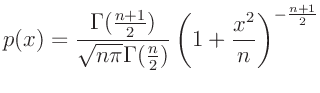
... t-Verteilung⁷

Standard t-Verteilung $x \sim t_n$ (z.B.Fahrmeir (2009) Seite 461)

$$p(x) = \frac{\Gamma(\frac{n+1}{2})}{\sqrt{n\pi}\Gamma(\frac{n}{2})} \left(1+\frac{x^2}{n}\right)^{-\frac{n+1}{2}}$$

.
.
.
.
.
.
.
.
.
.
.
.
.
.
.
.
.
.
.
.
.
.
.
.
.
.
.
.
.
.

... bestimmt.⁸

Zu bedingten Wahrscheinlichkeiten und zum Bayes-Theorem siehe z.B. Koch (2000) (Kapitel 2) oder Wakefield (2013) Kapitel 3

.
.
.
.
.
.
.
.
.
.
.
.
.
.
.
.
.
.
.
.
.
.
.
.
.
.
.
.
.
.

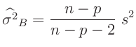
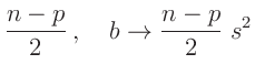
... wird.⁹

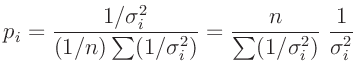
Die in den Gleichungen 10 und 11 genutzte, frei wählbare Konstante $c$ beeinflusst den Varianzfaktor $\sigma^2$, der auch als Varianz der Gewichtseinheit bezeichnet wird.

.
.
.
.
.
.
.
.
.
.
.
.
.
.
.
.
.
.
.
.
.
.
.
.
.
.
.
.
.
.

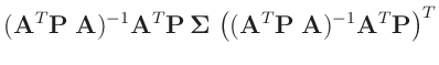
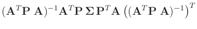
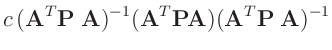
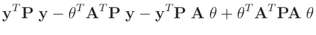
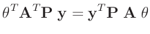
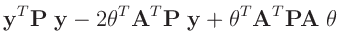
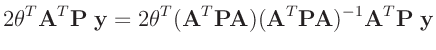
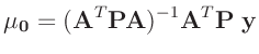
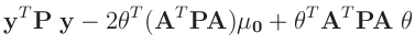
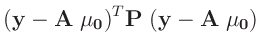
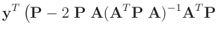
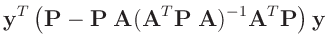
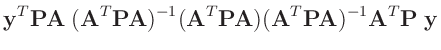
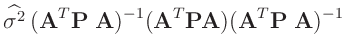
... umformen.¹⁰

Die Umformung erfolgt in mehreren Schritten. Dabei wird ausgenutzt, dass die Gewichtsmatrix $\bm{P}$ entsprechend ihrer Definition symmetrisch ist. Daraus ergibt sich , dass auch die Matrix $(\bm{A}^T\bm{P}\;\bm{A})$ symmetrisch ist.

$$(\bm{y}-\bm{A}\;\bm{\theta})^T\bm{P}(\bm{y}-\bm{A}\;\bm{\theta}) = \bm{y}^T\bm{P}\;\bm{y} - \bm{\theta}^T\bm{A}^T\bm{P}\;\bm{y} - \bm{y}^T\bm{P}\;\bm{A}\;\bm{\theta} + \bm{\theta}^T\bm{A}^T\bm{P}\bm{A}\;\bm{\theta}$$

$$\rightarrow \bm{\theta}^T\bm{A}^T\bm{P}\;\bm{y} = \bm{y}^T\bm{P}\;\bm{A}\;\bm{\theta}$$ alle Terme sind Skalare

$$= \bm{y}^T\bm{P}\;\bm{y} - 2 \bm{\theta}^T\bm{A}^T\bm{P}\;\bm{y} + \bm{\theta}^T\bm{A}^T\bm{P}\bm{A}\;\bm{\theta}$$

$$2\bm{\theta}^T\bm{A}^T\bm{P}\;\bm{y} = 2\bm{\theta}^T(\bm{A}^T\bm{P}\bm{A})(\bm{A}^T\bm{P}\bm{A})^{-1}\bm{A}^T\bm{P}\;\bm{y}$$ mit:

$$\bm{\mu_0}=(\bm{A}^T\bm{P}\bm{A})^{-1}\bm{A}^T\bm{P}\;\bm{y}$$ und:

$$= \bm{y}^T\bm{P}\;\bm{y} - 2\bm{\theta}^T(\bm{A}^T\bm{P}\bm{A})\bm{\mu_0} + \bm{\theta}^T\bm{A}^T\bm{P}\bm{A}\;\bm{\theta}$$ setze:

$$\bm{y}^T\bm{P}\,\bm{y} = \bm{y}^T\bm{P}\,\bm{y} -\bm{y}^T\bm{P}\bm{A}\;(\bm{A}^T\bm{P}\bm{... ...\bm{y} +\bm{y}^T\bm{P}\bm{A}\;(\bm{A}^T\bm{P}\bm{A})^{-1}\bm{A}^T\bm{P}\;\bm{y}$$

$$= \bm{y}^T\left(\bm{P}-\bm{P}\;\bm{A}(\bm{A}^T\bm{P}\;\bm{A})^{-1}\... ...\bm{y} +\bm{y}^T\bm{P}\bm{A}\;(\bm{A}^T\bm{P}\bm{A})^{-1}\bm{A}^T\bm{P}\;\bm{y}$$ aus

$$(\bm{y}-\bm{A}\;\bm{\mu_0})^T\bm{P}\;(\bm{y}-\bm{A}\;\bm{\mu_0}) = (\bm{y}-\bm{A}\;(\bm{A}^T\bm{P}\;\bm{A})^{-1}\bm{A}^T\bm{P}\;\bm{y})^T\bm{P}\; (\bm{y}-\bm{A}(\bm{A}^T\bm{P}\bm{A})^{-1}\bm{A}^T\bm{P}\;\bm{y})$$

$$= \bm{y}^T\left(\bm{I}-\bm{P}\;\bm{A}(\bm{A}^T\bm{P}\;\bm{A})^{-1}\... ...{P}\; \left(\bm{I}-\bm{A}(\bm{A}^T\bm{P}\bm{A})^{-1}\bm{A}^T\bm{P}\right)\bm{y}$$

$$= \bm{y}^T\left( \bm{P}-2\;\bm{P}\;\bm{A}(\bm{A}^T\bm{P}\;\bm{A})^{-1}\bm{A}^T\bm{P}\right.$$

$$\left.\hspace{12mm} +\;\bm{P}\;\bm{A}(\bm{A}^T\bm{P}\;\bm{A})^{-1}\bm{A}^T\bm{P}\;\bm{A} (\bm{A}^T\bm{P}\bm{A})^{-1}\bm{A}^T\bm{P} \right)\bm{y}$$

$$= \bm{y}^T\left( \bm{P}-\bm{P}\;\bm{A}(\bm{A}^T\bm{P}\;\bm{A})^{-1}\bm{A}^T\bm{P}\right)\bm{y}$$ und

$$\bm{y}^T\bm{P}\bm{A}\;(\bm{A}^T\bm{P}\bm{A})^{-1}\bm{A}^T\bm{P}\;\bm{y} = \bm{y}^T\bm{P}\bm{A}\;(\bm{A}^T\bm{P}\bm{A})^{-1}(\bm{A}^T\bm{P}\bm{A})(\bm{A}^T\bm{P}\bm{A})^{-1}\bm{A}^T\bm{P}\;\bm{y}$$

$$= \bm{\mu_0}^T(\bm{A}^T\bm{P}\bm{A})\bm{\mu_0}$$

$$(n-p)\;s^2 = (\bm{y}-\bm{A}\;\bm{\mu_0})^T\bm{P}\;(\bm{y}-\bm{A}\;\bm{\mu_0})$$ folgt mit:

$$\bm{y}^T\bm{P}\,\bm{y} = (n-p)\;s^2 + \bm{\mu_0}^T(\bm{A}^T\bm{P}\bm{A})\bm{\mu_0}$$ damit ergibt sich:

$$(\bm{y}-\bm{A}\;\bm{\theta})^T\bm{P}(\bm{y}-\bm{A}\;\bm{\theta}) = (n-p)\;s^2 + \bm{\mu_0}^T(\bm{A}^T\bm{P}\bm{A})\bm{\mu_0} - 2\bm{... ...bm{A}^T\bm{P}\bm{A})\bm{\mu_0} + \bm{\theta}^T\bm{A}^T\bm{P}\bm{A}\;\bm{\theta}$$

$$= (n-p)\;s^2 +(\bm{\theta}-\bm{\mu_0})^T\bm{A}^T\bm{P}\bm{A}\,(\bm{\theta}-\bm{\mu_0})$$

.
.
.
.
.
.
.
.
.
.
.
.
.
.
.
.
.
.
.
.
.
.
.
.
.
.
.
.
.
.

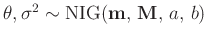
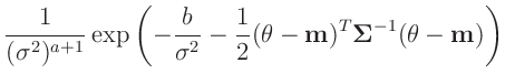
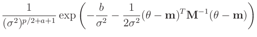
... Gammaverteilung¹¹

Normal-inverse Gamma-Verteilung $\bm{\theta},\sigma^2 \sim \mathrm{NIG}(\bm{m},\,\bm{\Sigma},\,a,\,b)$
(z.B. Fahrmeir (2013) Seite 652):

$$p(\bm{\theta},\sigma^2) = \frac{1}{(2\pi)^{p/2}\vert\bm{\Sigma}\vert^{1/2}}\frac{b^a}{\Gamma(a)}$$

$$\frac{1}{(\sigma^2)^{a+1}}\exp\left( -\frac{b}{\sigma^2} - \frac{1}{2} (\bm{\theta} - \bm{m})^T \bm{\Sigma}^{-1}(\bm{\theta} - \bm{m})\right)$$

Für die praktische Anwendung wird oftmals $\bm{\Sigma}=\sigma^2\,\bm{M}$ gesetzt und
$\bm{\theta},\sigma^2 \sim \mathrm{NIG}(\bm{m},\,\bm{M},\,a,\,b)$ verwendet (z.B. Fahrmeir (2013) Seite 227).

$$p(\bm{\theta},\sigma^2) = \frac{1}{(2\pi)^{p/2}\vert\bm{M}\vert^{1/2}}\frac{b^a}{\Gamma(a)}$$

$$\frac{1}{(\sigma^2)^{p/2+a+1}}\exp\left( -\frac{b}{\sigma^2} - \f... ...1}{2\sigma^2} (\bm{\theta} - \bm{m})^T \bm{M}^{-1}(\bm{\theta} - \bm{m})\right)$$

.
.
.
.
.
.
.
.
.
.
.
.
.
.
.
.
.
.
.
.
.
.
.
.
.
.
.
.
.
.

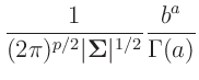
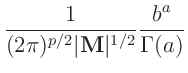
... Gamma-Verteilung¹²

Inverse Gamma-Verteilung $x \sim \mathrm{InvGa}(a,b)$
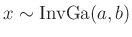
(z.B. Fahrmeir (2009) Seite 461):

$$p(x) = \frac{b^a}{\Gamma(a)}x^{-(a+1)}\exp(-b/x),\hspace{3mm}x>0$$

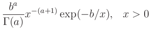$$\bm{\mathrm{E}}[x] = \frac{b}{a-1}$$ mit:

$$\rightarrow \int p(x)\;d x = 1$$ es gilt:

$$\rightarrow \int x^{-(a+1)}\exp(-b/x)\;d x = \Gamma(a)\;b^{-a}$$ daraus folgt:

.
.
.
.
.
.
.
.
.
.
.
.
.
.
.
.
.
.
.
.
.
.
.
.
.
.
.
.
.
.

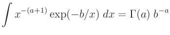... t-Verteilung¹³

$p$-dimensionale t-Verteilung $\bm{x} \sim \mathrm{T}_p(\bm{\mu},\bm{\Sigma},d)$
(z.B. Fahrmeir (2009) Seite 467)

$$p(\bm{x}) = \frac{\Gamma[(d+p)/2]}{\Gamma[d/2](d\;\pi)^{p/2}}\v... ...ac{(\bm{x}-\bm{\mu})^T\bm{\Sigma}^{-1}(\bm{x}-\bm{\mu})}{d}\right]^{-(d+p)/2}$$

.
.
.
.
.
.
.
.
.
.
.
.
.
.
.
.
.
.
.
.
.
.
.
.
.
.
.
.
.
.

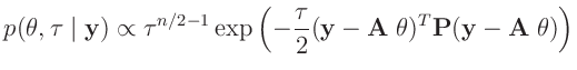
... Priori-Verteilungen¹⁴

Zu der gleichen Verteilung $\bm{\theta} \mid \bm{y}$ gelangt Koch (2000)( Seite 111 ff) mit einer anderen Priori-Verteilung. Er substituiert den Varianzfaktor $\sigma^2$ mit dem Gewichtsparameter $\tau = 1 / \sigma^2$ und benutzt die Priori-Verteilungen

$$p(\bm{\theta}) \propto const \hspace{5mm} -\infty < \theta_i < \infty\;,\; i=1,\ldots,n$$

$$p(\tau) \propto \tau^{-1} \hspace{5mm} 0 < \tau < \infty$$

$$p(\bm{\theta},\tau) = p(\bm{\theta})\times p(\tau) \propto \tau^{-1}$$

Daraus ergibt sich die Posteriori-Verteilung zu:

$$p(\bm{\theta},\tau\mid\bm{y}) \propto \tau^{n/2-1} \exp\left(-\fr... ...tau}{2}(\bm{y}-\bm{A}\;\bm{\theta})^T\bm{P}(\bm{y}-\bm{A}\;\bm{\theta})\right)$$

Der Exponent wird in der gleichen Weise umgeformt. Damit lässt sich die Posteriori-Verteilung als Normal-Gammaverteilung darstellen. Aus dieser folgt dann die mehrdimensionale t-Verteilung:

$$\bm{\theta} \mid \bm{y} \sim \mathrm{T}_p\left(\bm{\mu_0},\,s^2(\bm{A}^T\bm{P}\bm{A})^{-1}\,,\,n-p\right)$$

als Posteriori-Randverteilung für $\bm{\theta}$.

.
.
.
.
.
.
.
.
.
.
.
.
.
.
.
.
.
.
.
.
.
.
.
.
.
.
.
.
.
.

...,¹⁵

Fahrmeir (2013)(Seite 227ff.) verwendete als konjugierte Priori-Verteilung eine Normal-inverse Gammaverteilung $\theta,\sigma^2 \sim \mathrm{NIG}(\bm{m},\,\bm{M},\,a,\,b)$. Aus dieser folgt als Posteriori-Verteilung wieder eine Normal-inverse Gammaverteilung. Mit den von Fahrmeir (2013) auf Seite 231 angegebenen Werten $\bm{m} = \bm{0}$, $\bm{M}^{-1}=\bm{0}$, $a=-p$ und $b=0$ folgt als Priori-Verteilung:

$$p(\bm{\theta},\sigma^2) \propto \frac{1}{(\sigma^2)^{-p/2+1}} = (\sigma^2)^{p/2-1}$$

die nicht mit der von Fahrmeir (2013)(Gleichung. 4.16) angestrebten, nichtinformativen Priori-Verteilung

$$p(\bm{\theta},\sigma^2) \propto \frac{1}{\sigma^2}$$

übereinstimmt. Diese ist mit der Vorgabe $a=-p/2$ zu erreichen. Daraus ergibt sich dann als Posteriori-Verteilung

$$p(\bm{\theta},\sigma \mid \bm{y}) \propto \frac{1}{(\sigma^2)^{n... ...ma^2}(\bm{y}-\bm{A}\;\bm{\theta})^T\bm{P}\,(\bm{y}-\bm{A}\;\bm{\theta})\right)$$

die sich durch die Normal-inverse Gammaverteilung 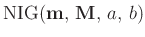$\mathrm{NIG}(\bm{m},\,\bm{M},\,a,\,b)$ mit

$$\hspace{5mm} \bm{m} \rightarrow \bm{\mu_0}\,\mathrm{,}\hspace{12mm} \bm{M} \rightarrow (\bm{A}^T\bm{P}\;\bm{A})^{-1}$$

$$\hspace{7mm} a \rightarrow \frac{n-p}{2}\,\mathrm{,}\hspace{5mm} b \rightarrow \frac{n-p}{2}\;s^2$$

beschreiben lässt.

.
.
.
.
.
.
.
.
.
.
.
.
.
.
.
.
.
.
.
.
.
.
.
.
.
.
.
.
.
.

... werden¹⁶

Wakefield (2013)(Seite 222) kommt auf eine inverse Chi Quadrat Verteilung mit $n-p$ Freiheitsgraden

$$\sigma^2\mid\bm{y} \sim (n-p)\;s^2 \times\chi^{-2}_{n-p}$$

wobei zu beachten ist, dass Wakefield (2013) den Parametervektor $\bm{\theta}$ von $0 \ldots k = p_W-2$ indiziert und dort in $p_W$, der Anzahl der unbekannten Parameter, $\sigma$ enthalten ist (Seite 209).
Der Erwartungswert der inversen Chi Quadrat Verteilung mit k Freiheitsgraden ist gegeben durch

$$\bm{\mathrm{E}}[\chi^{-2}_k] =\frac{1}{k-2}$$

Daraus folgt:

$$\widehat{\sigma^2}_B = \frac{n-p}{n-p-2}\;s^2$$

.
.
.
.
.
.
.
.
.
.
.
.
.
.
.
.
.
.
.
.
.
.
.
.
.
.
.
.
.
.

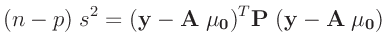
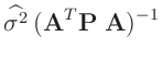
... abgeleitet¹⁷

Bei der Herleitung wird ausgenutzt, dass die Matrizen $\bm{P}$ und $\bm{A}^T\bm{P}\;\bm{A}$ symmetrisch sind.

$$\bm{\mathrm{Cov}}[\bm{\theta}] = \bm{H}\,\bm{\Sigma}\,\bm{H}^T$$

$$= (\bm{A}^T\bm{P}\;\bm{A})^{-1}\bm{A}^T\bm{P}\,\bm{\Sigma}\, \left((\bm{A}^T\bm{P}\;\bm{A})^{-1}\bm{A}^T\bm{P}\right)^T$$

$$= (\bm{A}^T\bm{P}\;\bm{A})^{-1}\bm{A}^T\bm{P}\,\bm{\Sigma}\, \bm{P}^T\bm{A}\left((\bm{A}^T\bm{P}\;\bm{A})^{-1}\right)^T$$

$$\mathrm{mit:} \hspace{4mm}\bm{\Sigma} = c\;\bm{P}^{-1}$$

$$= c\,(\bm{A}^T\bm{P}\;\bm{A})^{-1}(\bm{A}^T\bm{P}\bm{A})(\bm{A}^T\bm{P}\;\bm{A})^{-1}$$

$$= c\,(\bm{A}^T\bm{P}\;\bm{A})^{-1}$$

.
.
.
.
.
.
.
.
.
.
.
.
.
.
.
.
.
.
.
.
.
.
.
.
.
.
.
.
.
.